In our previous blog we studied about the basic concepts of Linear Regression and its assumptions and let’s practically try to understand how it works.
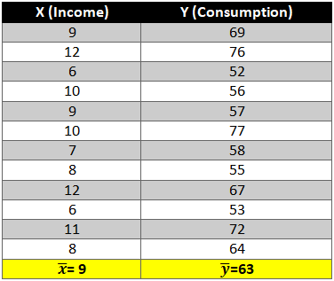
Given below is a dataset for which we will try to generate a linear function i.e.
y=b0+b1Xi
Where,
y= Dependent variable
Xi= Independent variable
b0 = Intercept (coefficient)
b1 = Slope (coefficient)
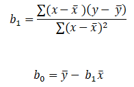
To find out beta (b0& b1) coefficients we use the following formula:-
Let’s start the calculation stepwise.
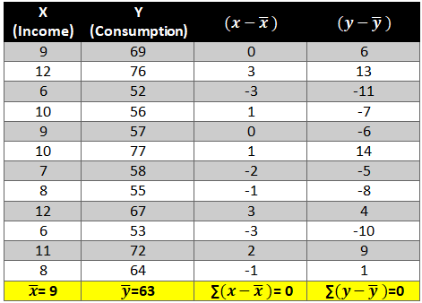
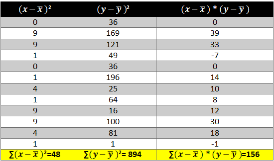
- First let’s find the mean of x and y and then find out the difference between the mean values and the Xi and Yie. (x-x ̅ ) and (y-y ̅ ).
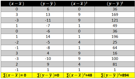
- Now calculate the value of (x-x ̅ )2 and (y-y ̅ )2. The variation is squared to remove the negative signs otherwise the summation of the column will be 0.
- Next we need to see how income and consumption simultaneously variate i.e. (x-x ̅ )* (y-y ̅ )
Now all there is left is to use the above calculated values in the formula:-
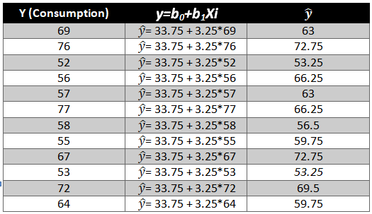
As we have the value of beta coefficients we will be able to find the y ̂(dependent variable) value.
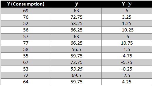
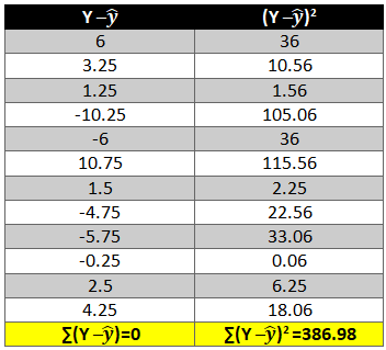
We need to now find the difference between the predicted y ̂ and observed y which is also called the error term or the error.
To remove the negative sign lets square the residual.
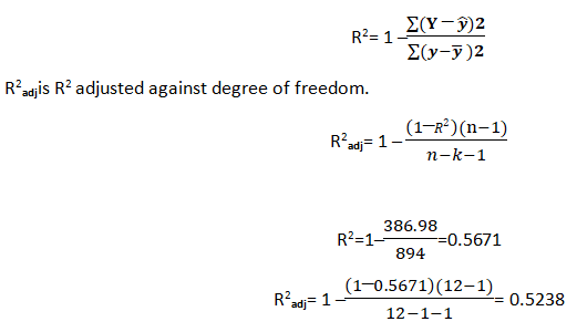
What is R2 and adjusted R2 ?
R2 also known as goodness of fit is the ratio of the difference between observed y and predicted and the observed y and the mean value of y.
Hopefully, now you have understood how to solve a Linear Regression problem and would apply what you have learned in this blog. You can also follow the video tutorial attached down the blog. You can expect more such informative posts if you keep on following the DexLab Analytics blog. DexLab Analytics provides data Science certification courses in gurgaon.
.

Comments are closed here.