Recently, a discussion was held, which invited data scientists and analysts all over the world, to take part in the Science of Super Bowl discussion panel, this discussion was held by Newswise.
We found one notable discussion topic, which answered three very important questions related to data science that the sports industry could use:
How data science works?
How can we use data science to help NFL?
How can the analytical outputs of data science affect the outcome of the Super Bowl?
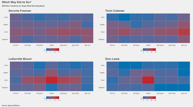
A few visuals created with R programming, can help to address these questions the best. The finished product to explain that is mentioned below:
A comprehensive R language training can help you create more such explanatory visuals of high quality for explaining complex topics. We are a reputable R predictive modelling training institute based in Delhi NCR and Pune that offer best in class R analytics certification.
######################################################
# RB direction charts
# 2/1/2017
#
#
######################################################

library(nflscrapR)
library(dplyr)
library(ggplot2)
library(ggthemes)
library(gtable)
library(grid)
library(gridExtra)

# download all paly by play data for 2016 including playoffs -----
# this is going to take a while
reg_games post_games all_games

game_list

s16

# calculate run percentages -----
rundf % filter(PlayType %in% c("Run") &
!is.na(down) &
posteam %in% c("NE", "ATL")) %>%
mutate(depth = ifelse(Yards.Gained <= 0, "Negative", "Short"), depth = ifelse(Yards.Gained >= 5, "Middle", depth),
depth = ifelse(Yards.Gained >= 10, "Deep", depth)) %>%
group_by(posteam, Rusher) %>%
mutate(down_n = n()) %>%
group_by(posteam, Rusher, RunLocation, RunGap, depth) %>%
summarise(play_per = (n() / mean(down_n)) * 100,
loc_att = n(),
total_att = mean(down_n))

# just a little clean up -----
rundf[is.na(rundf$RunLocation), "RunLocation"] <- "middle"
rundf[rundf$RunLocation == "middle", "RunGap"] <- ""

rundf$runplace

rundf$runplace "left guard", "middle",
"right guard", "right tackle",
"right end"))

rundf$depth

# not all RBs will have runs to all locations, so make a full data frame -----
# and join to it before charting
fulldf "middle", "right guard", "right tackle",
"right end"),
"depth" = c("Negative", "Short", "Middle", "Deep"))

# Devonta Freeman -----
freemandf % filter(Rusher == "D.Freeman") %>%
right_join(fulldf) %>% mutate(play_per = ifelse(is.na(play_per), 0, play_per))

freeman_plot geom_tile(aes(fill = play_per),colour = "white") +
scale_fill_gradient(high = "#ca0020", low = "#0571b0",
limits = c(0,15), guide_colourbar(title = "%")) +
theme_fivethirtyeight() +
labs(title = "Devonta Freeman")

# Dion Lewis -----
lewisdf % filter(Rusher == "D.Lewis") %>%
right_join(fulldf) %>% mutate(play_per = ifelse(is.na(play_per), 0, play_per))

lewis_plot geom_tile(aes(fill = play_per),colour = "white") +
scale_fill_gradient(high = "#ca0020", low = "#0571b0",
limits = c(0,30), guide_colourbar(title = "%")) +
theme_fivethirtyeight() +
labs(title = "Dion Lewis")

# blount -----
blountdf % filter(Rusher == "L.Blount") %>%
right_join(fulldf) %>% mutate(play_per = ifelse(is.na(play_per), 0, play_per))

blount_plot geom_tile(aes(fill = play_per),colour = "white") +
scale_fill_gradient(high = "#ca0020", low = "#0571b0",
limits = c(0,15), guide_colourbar(title = "%")) +
theme_fivethirtyeight() +
labs(title = "LeGarrette Blount")
To learn further about such coding in R programming take up R programming courses in Gurgaon.
# Devonta Freeman -----
freemandf % filter(Rusher == "D.Freeman") %>%
right_join(fulldf) %>% mutate(play_per = ifelse(is.na(play_per), 0, play_per))

freeman_plot geom_tile(aes(fill = play_per),colour = "white") +
scale_fill_gradient(high = "#ca0020", low = "#0571b0",
limits = c(0,15), guide_colourbar(title = "%")) +
theme_fivethirtyeight() +
labs(title = "Devonta Freeman")

# Dion Lewis -----
lewisdf % filter(Rusher == "D.Lewis") %>%
right_join(fulldf) %>% mutate(play_per = ifelse(is.na(play_per), 0, play_per))

lewis_plot geom_tile(aes(fill = play_per),colour = "white") +
scale_fill_gradient(high = "#ca0020", low = "#0571b0",
limits = c(0,30), guide_colourbar(title = "%")) +
theme_fivethirtyeight() +
labs(title = "Dion Lewis")

# blount -----
blountdf % filter(Rusher == "L.Blount") %>%
right_join(fulldf) %>% mutate(play_per = ifelse(is.na(play_per), 0, play_per))

blount_plot geom_tile(aes(fill = play_per),colour = "white") +
scale_fill_gradient(high = "#ca0020", low = "#0571b0",
limits = c(0,15), guide_colourbar(title = "%")) +
theme_fivethirtyeight() +
labs(title = "LeGarrette Blount")

# colemen -----
colemandf % filter(Rusher == "T.Coleman") %>%
right_join(fulldf) %>% mutate(play_per = ifelse(is.na(play_per), 0, play_per))

coleman_plot geom_tile(aes(fill = play_per),colour = "white") +
scale_fill_gradient(high = "#ca0020", low = "#0571b0",
limits = c(0,15), guide_colourbar(title = "%")) +
theme_fivethirtyeight() +
labs(title = "Tevin Coleman")

# combine plots and add text -----

p1 blount_plot, lewis_plot)

# sub title ----
titleback titlesub gp = gpar(fontsize = 12, fontface = "bold",
fontfamily = "sans", col = "#3C3C3C"),
just = "left", x = unit(0.01, "npc"))

padding

p1 p1

# title ----
title gp = gpar(fontsize = 18, fontface = "bold",
fontfamily = "sans", col = "#3C3C3C"),
just = "left", x = unit(0.01, "npc"))

p1 p1

# bottom ----
subtext gp = gpar(fontsize = 10, fontface = "bold.italic",
fontfamily = "sans", col = "#3C3C3C"),
just = "left", x = unit(0.01, "npc"))

p1 p1 b = nrow(p1), r = 2)
grid.draw(p1)

ggsave(plot = p1, filename = "plots/rb direction.png",
width = 18, height = 10, units = "in", dpi = 600)
For more interesting tutorials and tips on R programming or a coveted Data Science Online Learning, feel free to contact our domain-based experts at DexLab Analytics.
Interested in a career in Data Analyst?
To learn more about Machine Learning Using Python and Spark – click here.
To learn more about Data Analyst with Advanced excel course – click here.
To learn more about Data Analyst with SAS Course – click here.
To learn more about Data Analyst with R Course – click here.
To learn more about Big Data Course – click here.
Big data certification pune, data analytics, data science, R Programming, R programming certification, SAS Courses and R


Comments are closed here.