Here is taking an in-depth look at how sampling distribution works along with a discussion on various types of the sampling distribution. This is a continuation of the discussion on Classical Inferential Statistics that focused on the theory of sampling, breaking it down to building blocks of classical sampling theory along with various kinds of sampling. You can read part 1 of the article here
Contents:
- Introduction
- Probability Density Function, Moment Generating Function, Sampling Distribution, Degrees of Freedom
- Gamma Function, Beta Function, Relation between Gamma & Beta Function
- Gamma Distribution
- Beta Distribution
- Chi-square Distribution & Exponential Distribution
- T-Distribution & F-Distribution
1. Introduction
The sampling distribution is a probability distribution of statistics obtained from a large number of samples drawn from a specific population. And the types of sampling distribution are- (i) Gamma Distribution, (ii) Beta Distribution, (iii) Chi-Square Distribution, (iv) Exponential Distribution, (v) T-Distribution & (vi) F-Distribution.
The key components for describing all these distributions are – (i) Probability Density Function – Which is the function whose integral is to be calculated to find probabilities associated with a continuous random variable and their shape(graph) for the same, (ii) Moment Generating Function – which helps to find the moment of those distributions, and (iii) Degrees of Freedom – It refers to the number of independent sample points and compute a static minus the number of parameters explained from the sample.
For Gamma and Beta distribution, we will discuss gamma and beta function and relation between them etc.
2. Probability Density Function, Moment Generating Function, Sampling Distribution, Degrees of Freedom
PROBABILITY DENSITY FUNCTION
Probability density function (PDF), in statistics, is a function whose integral is calculated to find probabilities associated with a continuous random variable (see continuity; probability theory). Its graph is a curve above the horizontal axis that defines a total area, between itself and the axis, of 1. The percentage of this area included between any two values coincides with the probability that the outcome of an observation described by the probability density function falls between those values. Every random variable is associated with a probability density function (e.g., a variable with a normal distribution is described by a bell curve). If X be continuous Random variable taking any continuous real values then f(x) is a probability density function if:-
Moment Generating Function
The moment generating function (m.g.f.) of a random variable X (about origin) having the probability function f(x) is given by:
The integration of summation being extended to the entire range of x, t being the real parameter and it is being assumed that the right-hand side of the equation is absolutely convergent for some positive number h such that –h<t<h.
SAMPLING DISTRIBUTION
It may be defined as the probability law which the statistic follows if repeated random samples of a fixed size are drawn from a specified population. A number of samples, each of size n, are taken from the same population and if for each sample the values of the statistic are calculated, a series of values of the statistic will be obtained. If the number of samples is large, these may be arranged into a frequency table. The frequency distribution of the statistic that would be obtained if the number of samples, each of the same size (say n), were infinite is called the Sampling distribution of the statistic
DEGREES OF FREEDOM
The term degrees of freedom (df) refers to the number of independent sample points used to compute a statistic minus the number of parameters estimated from the sample points: For example, consider the sample estimate of the population variance (s2)
Where is the score for observation i in the sample, X ̅ is the sample estimate of the population mean, n is the number of observation in the sample. The formula is based on n independent sample points and one estimated population parameter (x ̅). Therefore, the number of degrees of freedom is n minus one. For this example
df=n-1
3. Gamma Function, Beta Function, Relation between Gamma &Beta Function
GAMMA FUNCTION
The Gamma function is defined for x>0 in integral form by the improper integral known as Euler’s integral of the second kind.
Many probability distributions are defined by using the gamma function, such as gamma distribution, beta distribution, chi-squared distribution, student’s t-distribution, etc. For data scientists, machine learning engineers, researchers, the Gamma function is probably one of the most widely used functions because it is employed in many distributions.
BETA FUNCTION
The Beta function is a function of two variables that is often found in probability theory and mathematical statistics.
The Beta function is a function B: R_(++)^2→R defined as follows:
There is also a Euler’s integral of the first kind.
For example, as a normalizing constant in the probability density functions of the F distribution and of the Student’s t distribution
RELATION BETWEEN GAMMA AND BETA FUNCTION
In the realm of Calculus, many complex integrals can be reduced to expressions involving the Beta Function. The Beta Function is important in calculus due to its close connection to the Gamma Function which is itself a generalization of the factorial function.
We know,
So, the product of two factorials as
Now apply the changes of variables t=xy and s=x(1-y) to this double integral. Note that t + s = x and that 0 < t < ∞ and 0 < x < ∞ and 0 < y < 1. The jacobian of this transformation is
Since x > 0 we conclude that  Hence we have
Therefore,
4. Gamma Distribution
The gamma distribution is a widely used distribution. It is a right-skewed probability distribution. These distributions are useful in real life where something has a natural minimum of 0.
If X be a continuous random variable taking only positive values, then X is said to be following a gamma distribution iff its p.d.f can be expressed as:- 
=0 otherwise….(1)
- Probability Density Function for Gamma Distribution
For (1), to be the Probability Density Function, we must have:-
Now, f(x)>0 if x>0 & f(x)=0 if x taking any non-positive values, so, f(x)≥0 ∀x .
Hence, condition (i) is satisfied. Now,
Using (3) & (4) in (2) we get:-
Hence, f(x) statistics condition (ii).
So, equation (1) is a proper pdf.
- Moment Generating Function for Gamma Distribution
Moment generating functions are general procedure of finding out moments of a probability distribution mathematically it may be expressed as- M_x (t)=E(e^xt )
This represents raw moments of the random variable X about to the origin 0.
Three important properties of m.g.f. are:- (i) where c is a constant.(ii) If ’s are independent Random variables i.e. then (iii) If X and Y are two random variables and if then X and Y are two identical distribution this is called the uniqueness property,Calculating the m.g.f. of gamma distribution:
Using (2) and (3) in (1) we get:
5. Beta Distribution
In probability theory and statistics, the beta distribution is a family of continuous probability distributions defined on the interval [0, 1] parameterized by two positive shape parameters, denoted by α and β, that appear as exponents of the random variable and control the shape of the distribution.
The beta distribution has been applied to model the behavior of random variables limited to intervals of finite length in a wide variety of disciplines.
- Probability Density Function for Beta Distribution
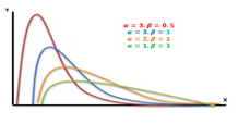
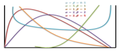
The probability density function (PDF) of the beta distribution, for 0 ≤ x ≤ 1, and shape parameters α, β > 0, is a power function of the variable x and of its reflection (1 − x) as follows:
Where Γ(z) is the gamma function. The beta function, B, =+is a normalization constant to ensure that the total probability integrates to 1. In the above equations, x is a realization—an observed value that actually occurred—of a random process X.
This definition includes both ends x = 0 and x = 1, which is consistent with the definitions for other continuous distributions supported on a bounded interval which are special cases of the beta distribution, for example, the arcsine distribution, and consistent with several authors, like N. L. Johnson and S. Kotz. However, the inclusion of x= 0 and x= 1 does not work for α, β < 1; accordingly, several other authors, including W. Feller, choose to exclude the ends x = 0 and x = 1, (so that the two ends are not actually part of the domain of the density function) and consider instead 0 < x < 1. Several authors, including N. L. Johnson and S. Kotz, use the symbols p and q (instead of α and β) for the shape parameters of the beta distribution, reminiscent of the symbols are traditionally used for the parameters of the Bernoulli distribution, because the beta distribution approaches the Bernoulli distribution in the limit when both shape parameters α and β approach the value of zero.
In the following, a random variable X beta-distributed with parameters α and β will be denoted by:
Other notations for beta-distributed random variables used in the statistical literature are. X- Be(α,β)and X~β_(α,β)
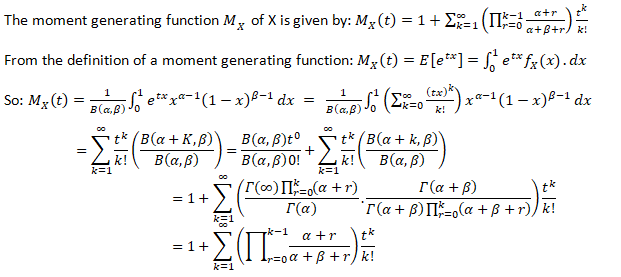
- Moment Generating Function for Beta Distribution
6. Chi-square Distribution & Exponential Distribution
CHI-SQUARE DISTRIBUTION
A chi-square distribution is defined as the sum of the squares of standard normal variates. Let x be a random variable which follows normal distribution with mean μ& variance  then standard normal variate is defined as: –
 ![]()
The variate Z is said to follow a standard normal distribution with mean 0 and variance 1. Let X be a random variable containing observations,![]() .
.
Then the chi-square distribution is defined as:- ![]() So we can say:-
So we can say:-
A chi-square distribution with ‘n’ degree of freedom, where degrees of freedom refer to number of independent associations among variables.
- The Probability Density Function of a Chi-Square Distribution:
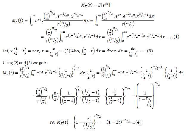
The Moment Generating Function of Chi-Square Distribution:
(4) is a required m.g.f. of the chi-square distribution.
EXPONENTIAL DISTRIBUTION
The Exponential distribution is one of the widely used continuous distributions. It is often used to model the time elapsed between events.
The Probability Density Function of Exponential Distribution:
Let X be a continuous random variable assuming only real values then X is said to be following an exponential distribution iff:-
Therefore, exponential distribution is a special case of gamma
distribution with v = 1.
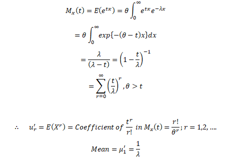
- The Moment Generating Function of Exponential Distribution:
Let X~Exponential (λ), we can find its expected value as follows, using integration by parts:
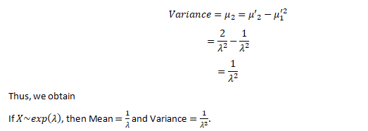
Now let’s find Var (X), we have
7. T-Distribution & F-Distribution
T-DISTRIBUTION
Student’s t-distribution:
If x1,x2,… ,xn be ‘n’ random samples drawn from a normal population having mean & standard deviation then the statistics following student t-distribution with (n-1) degrees of freedom.
Fisher’s t-distribution:
Let X~N(0,1) & let the random variable Y~X_n^2. Both X & Y are independent random variables. Then the fisher’s t-distribution is defined as :-
Probability Density Function for t-distribution:
Where, t2 > 0 Where, v=(n-1) degrees of freedom
= 0 , otherwise
For Fisher’s t-distribution:
Where, t2 > 0
=0 otherwise
Application of t-distribution:
If x1,x2, and x3 are independent random variables. Each following a standard normal distribution. What will be the distribution of ![]()
F- DISTRUBUTION
The F-Distribution is a ration of two chi-square distributions. If X be a random variable which follows a fisher’s t-distribution.Then:- ![]()
Squaring the above expression we get:
The R.V. X2~F1, n. Then we say X2 follows F-distribution with 1,n degrees of freedom.
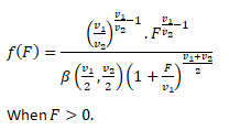
- Probability Density Function for F-distribution:
- Application of F-Distribution:
Let x1,x2,… ,xn be a random sample drawn from a normal population with mean μ & variance σ2. where both μ & σ are unknown. Obtain the MLEs of θ.
Let x1,x2,… ,xn be ‘n’ random sample drawn from a normal population with mean μ & variance σ2.
Taking logarithms on both sides; we get:-
CONCLUSION: That was a thorough analysis of different types of sampling distribution along with their distinct functions and interrelations. If the resource was useful in understanding statistical analytics, find more such informative and analytical, subject-oriented discussion regarding statistical analytics courses on DexLab Analytics blog.
.













Comments are closed here.